First steps of fitting

There is a preferable order of which parameters should be fitted when. Patience is advisory; as you gain experience, you will get the feeling of how to approach to certain types of problems. But the usual recipe would be this: start with luminosities. These quantities, although carrying physical name, are actually "normalizers" of your experimental data; original minimization routines work with fluxes, not with magnitudes, so PHOEBE internally does all the necessary conversions. These conversions are based on the normalizing magnitude that is set in the Data tab. It defaults to 10, but should be set to the magnitude of the quarter phase; as this cannot (and shouldn't) be done too accurately, luminosities jump in and normalize the data so that the normalization is actually done internally and you don't have to worry about it. These luminosities are referred to as HLA and CLA in in WD.

Go to the Luminosities tab (Fig. 17) and turn on the Adjust HLAs switch. Leave the step as it is, since we are going to use Levenberg-Marquardt's $\lambda$ multiplicator routine, which automatically chooses a proper step size when close to the solution.

Figure 17: PHOEBE luminosities tab.

Now go to the Fitting tab (Fig. 18); the upper part of the tab is dedicated to the method of multiple subsets, which we will not use in this tutorial. The lower left part belongs to the two-dimensional projection of the parameter phase-space, which helps us analyse parameter correlations. We shall demonstrate its use in the course of this tutorial. On the right, there are fitting parameters, which are generally a good choice. Change grid sizes only if stellar shapes deviate significantly from spheroids, change Marquardt's $\lambda$ only if convergence isn't satisfactory. Choosing symmetrical derivatives is a better approximation, but at the expence of computing time. Since the time isn't that important at the moment, turn on symmetrical derivatives! After you have gotten yourself comfortable, click on the Fit Parameters Set For Adjustment switch!

Figure 18: PHOEBE fitting tab.

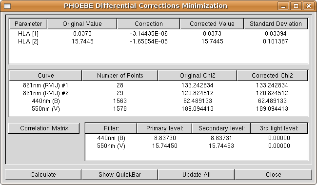
After you have clicked on that button, a fitting window (Fig. 19) will show up. This window is composed of three lists that contain important information for monitoring the progress of your soulution trough iterations.

Figure 19: PHOEBE differential corrections window.

On the top of the fitting window is a columned list that contains all parameters selected for adjustment. In case of curve-independent parameters there is only one entry and in case of curve-dependent parameters there are as many entries as there are affected curves. Light curves and radial velocity curves differ in this respect and have each their own adjustment switches.

Parameter names are followed by their current values. The fitting algorithm will calculate the correction of one iteration. Be very careful about these values, for they are the best marker to show if the fit converges or diverges. Luminosities essentially always converge, but you can never be too sure. This list also shows the corrected value and standard deviation of the fit of the particular parameter.

Next is a list of all experimantal curves detailing the number of points and the $\chi^2$ values before and after calculation for each curve. The $\chi^2$ values change after each iteration to reflect the similarity of the newly calculated curves to experimental data, and thus are another way to monitor the convergence of your soulution.

Finally, in the lower part of the fitting window there is a list of passband luminosities for the primary and secondary stars, as well as for the $3^\mathrm{rd}$ body.

Now click on the Calculate button! After some seconds of calculating (depending on the speed of your computer), the window as in Fig. 20 will show up.

Figure 20: PHOEBE differential corrections window with calculated parameters.

You may see that both corrections (and their corrected values) are in agreement with what we expect (recall what offsets we saw in plotting windows). Since we are happy with the fit results, we want to keep them. So click on Update all corrections button to replace the original values in both the fitting window and in the main PHOEBE window with corrected values. The fitting function is now ready for the second iteration, so click on Calculate button again! The corrections will now be even smaller and the convergence obvious. Update the corrected values and recalculate the values as many times as you see fit. As long as you are far away from the solution, be sure to let the values converge on a decimal or two, but as the fit gets better and better, try to be as accurate as possible. If you persisted completely through the convergence, you should have come up with these values:

Figure 21: PHOEBE differential corrections window with calculated parameters after several itterations.

Before you close the fitting window, take notice of the Show QuickBar button. It opens a window where you can mark any system parameter for adjustment and change its adjustment step. This is a time-saving shortcut worth of keeping in mind.

When you've finished (and are happy) with fitting, close the window by clicking on the Close button. Go to the Luminosities tab (or enter the Fitting QuickBar), turn off the adjustment switch of the luminosities and inspect the results, as you have before, for both light curves. Notice any difference? Still not perfect, but much better.